
The multiple regression analysis is a technique of multivariate statistical analysis that has the aim to determine the ratio among a variable regarded as “objective” of search (dependent variable) and a set of explanatory variables (or independent variables).
In practical terms, this technique is used to predict a future time series data in order to get assumptions or dependency relationships through the use of statistical inference.
In a case where the relationship between the variables involved was known with accuracy you could perfectly define the response of the dependent variable to the stresses of the explanatory variables, but this rarely happens especially in economic reality. It is so unusual to know all the relevant explanatory variables, also some of these variables can not be measured or are measured only with error and besides the functional form of the relationship might not be known. In other words, empirically, the relationship between the dependent variable and independent variables can be known in less than one error. To take account of these conditions, you must use probabilistic models: one of these models is precisely the Multiple Regression Model. A manager may be interested to know how sales of a particular product are related to it’s price, to competing products price or to the amount of investment; in a similar way, in the macroeconomic sphere, an economist may be interested in evaluating the elasticity of GDP to changes in government spending or private sector investment. Hence the time series data related to the price of a product or the elasticity of GDP, representing variables targeted, are the result of a cluster of explanatory variables such as prices offered by competitors or the costs of advertising in the first case, the public spending or private investment in the second case.
Accordingly, the goal of this article is to describe a concrete example of the application of the multiple regression model, treating the analysis of passengers carried by an airline on a route lasting about 1 hour. I thought of using a case related to the sector I work in, because I have tested in practice in my career.
I won’t reveal the name of the airline that I will identify with Y as well as the take-off and landing airports I’m going to identify with A and B.
Business Case:
Distribution of the quantitative dependent variable
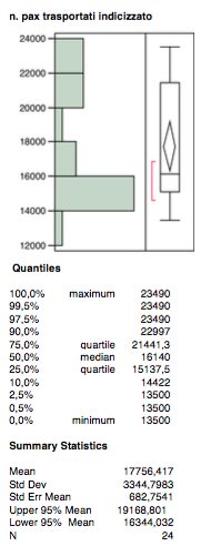
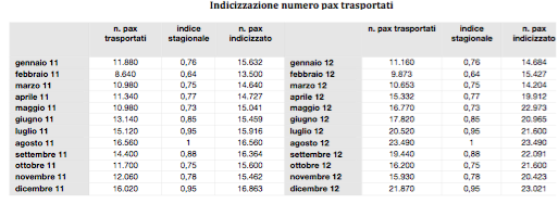
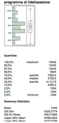
The number of pax transported on the route from A to B in the years 2011 and 2012 is the dependent variable on this analysis. It is indexed in order to sterilize the effect of seasonality that has considerable importance in the air transport business. More specifically, I have used standard indices published by IATA (International Air Transport Association), in order to mediate the flow of traffic during the months of the year according to the diagram in the model below.
The distribution of the variable appears quite balanced, there are no outliers.
The median tends to the 1st quartile and it touches the lower limit of the confidence interval, this means a marked difference between mean and median.
The interquartile range moves towards the observations located on the bottom wafer.
Distribution of quantitative independent variables
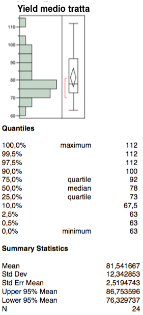
The first independent variable is represented by the “average yield” (net profit for each passenger).
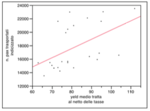
The distribution of the variable presents whole values between 105 and 110 as is evident in the chart on bivariate analysis with the dependent variable. From the correlation graph there are no phenomena of bi-modal distribution (Simpson paradox) there are no outliers.
The interquartile range tends to lower the wafer; the confidence interval appears quite centered with respect to interquartile interval. Finally, the median tends towards the first quartile well below the average.
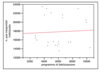
The second independent variable is related to investments regarding the “loyalty program“. They are the costs incurred for communication and for awarding tickets granted to passengers to achieve the score required by the regulation.
Also in this case the distribution is presented without outliers and there are no phenomena of bi-modal distribution as is shown by the graph below of the bivariate analysis.
As for the median, it is very close to the average, so the confidence interval appears very centered within interquartile range that appears quite symmetrical with respect to the distribution of the variable.
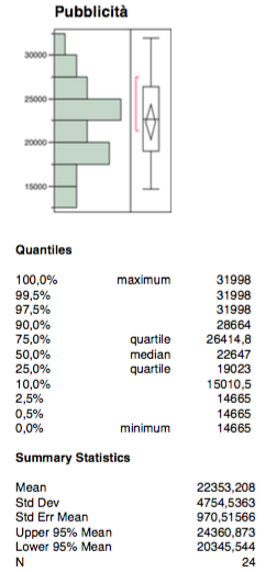
The third independent variable concerns the costs in communication media.
The distribution has no outliers and bi-modal phenomena, mean and median are close enough, the confidence interval and the interquartile range are quite focused on the distribution.
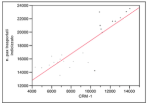
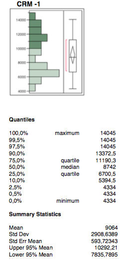
The fourth independent variable is CRM -1. It is referred to investment in direct communication towards the customer and more generally to customer care costs. Being a type of investment with no immediate effect, it is reasonable to see the effect the following month when it is operated. This is the meaning of -1.
The variable has no outliers but you may notice light phenomena of bi-modal distribution in the graph of the bi-variate analysis. For this reason the dichotomous variable “6 daily rate” was used in order to combine the two distributions.
Mean and median are far enough apart, both the interquartile range and the confidence interval tend to lower values of the distribution.
Distribution of dichotomous dependent variables
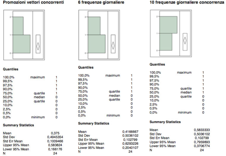
Le variabili dicotomiche si = 1 no = 0 sono connesse:
a) all’esistenza di promozioni in atto di vettori concorrenti sulla tratta;
b) al passaggio a 6 frequenze giornaliere dalle precedenti 4 anche a soluzione del fenomeno di bimodalità presente nella variabile CRM -1
c) al passaggio da parte delle concorrenza da 10 a 8 frequenze giornaliere
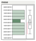
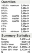
Distribuzione della variabile temporale
Come si evince dal grafico, la relazione tra numero pax trasportati e arco temporale, che ha nei mesi la propria unità di misura, non presenta fenomeni di distribuzione bimodale.
Dichotomous variables yes = 1 no = 0 are related to:
a) existence of promotions in place of competing carriers on the route;
b) passage from the previous 4 to 6 daily frequencies, also in solving the phenomenon of bi-modality in variable CRM -1
c) passage of the competitors from 10 to 8 daily frequencies
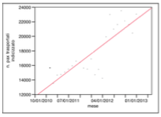
Distribution of the time variable
As can be seen from the graph, the relationship between the number of pax transported and time span, measured in month, is not affected by bi-modal distribution.
Correlation matrix between the variables
Scatterplot Matrix
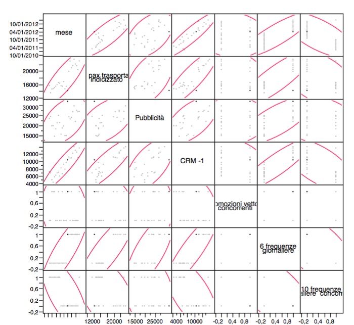
The correlation matrix presents some quite high values of ρ relative to the independent variables, this is also highlighted by the matrix scatterplot. Thus, it is the variable month, which has coefficients of relation higher than the other independent variables. At this point, in order to prevent an artificial increase in the explained variability and then the phenomenon of multicollinearity, we have to eliminate that variable, before local and global analysis.
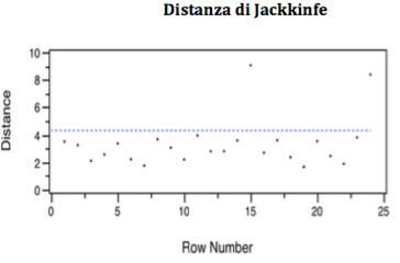
Multivariate analysis of outliers
According to the Mahalanobis distance, the analysis performed shows a certain constancy of the dissimilarity of the observations which remains almost the same.
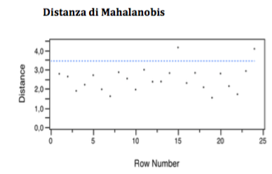
The Jakknife distance, in this case substantially confirms the Mahalanobis distance, so they have to be eliminated as outliers: observation n. 15 and also n. 24.
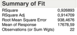
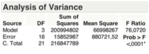
Analisi globale
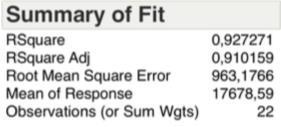
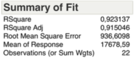
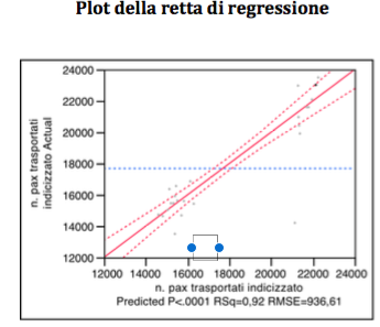
The value of R Square, considering the table below, shows a high degree of correlation between the variables, also confirmed by the value of R Square adjusted:
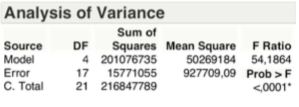
The F-Test (or Durbin-Watson Test), relative to the explained variance, allows us to reject the Ho hypothesis with a significance less than 1 x 1000, there is at least one β different from zero.
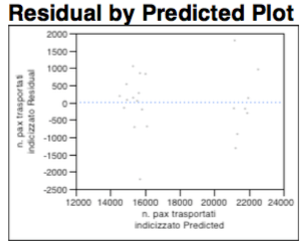
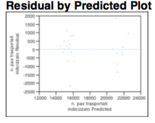
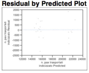
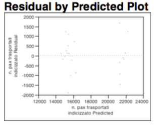
The residue analysis shows that the whole explained by the dichotomous variable relative to the “6 daily frequencies”, remains a random distribution of points, which does not imply the use of linear transformations. There are no phenomena of heteroskedasticity and “known geometric shapes” are not recognize. Finally the cloud appears randomly populated as shown in the graph below:
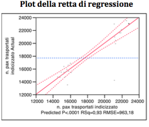
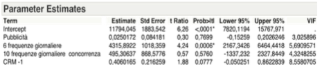
Local Analysis
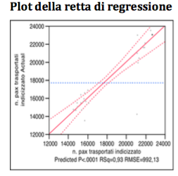
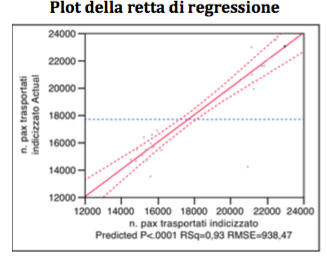
As highlighted by the plot of the regression line, the VIF > 10 concerns the variable CRM -1, because of the value of 12.5 we should not eliminate the variable. Thus, according to the Backward Method, the variable to be eliminated is: “promotion competing carriers”.
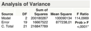
Global Analysis
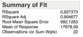
Following the elimination of the variable “promoting competing carriers”, the “Summary of Fit” below shows that R Square decreases slightly, while there is an increase in the value of R Square adjusted.
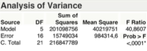
The F-test on the explained variance, as shown in the table below, is exceeded, so you can again reject the hypothesis Ho.
The diagram analysis of residues denotes a consolidation of the whole, again are not present phenomena of hetero-skedasticity or known geometric shapes.
Local Analysis
Following the elimination performed, the plot and table below show that the VIF variable CRM -1 is returned within the threshold defined by 10, the choice not to delete the variable we are getting is correct. It continues, according to the Backward Method, we can delete the variable “advertising”.
Global Analysis
The “Summary of Fit” shows that the value of R Square continues to decline slightly, while R Square adjusted, continues to increase:
The F-test on the explained variance, as shown in the table below is exceeded, therefore you can again reject the hypothesis Ho.
There are no substantial differences in the diagram of the residues, below.
Local Analysis
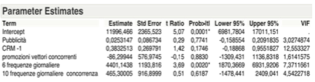
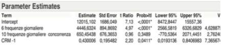
Following the Backward Method, as shown below, the diagram of the regression line and the table of estimated figures exclude the variable: “10 daily rate”
Global Analysis
The “Summary of Fit” shows that the value of R Square continues to decline, while R Square Adjusted continues to increase.
As shown in the table below, considering the F-test on the variance, we can still reject the hypothesis Ho.
There are no substantial differences in the diagram of residues.
Local Analysis
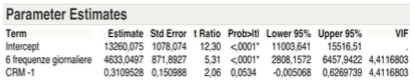
Even if the estimated parameters from the table below show a value slightly greater than the significance level of 5% of the variable CRM-1, it can be considered explanatory with respect to the variable target.
At the end of the analysis we have these local independent variables left:
1) 6 daily frequencies = X1
2) CRM-1 = X2
At this point of the analysis process, it is necessary to standardize the parameters relating to the two variables remaining at the end of the selection process by calculating the relative standard β. They are pure numbers compared to the values of the estimated parameters, because they are not affected by different units or different quantitative values of variables and they represent the weights of the remaining independent variables within the regression line function.
The table of the estimated parameters referred to in the last local analysis, shows the intercept equal to 13,260.08. The standardized value of X1 => β1 = 0.709884; the standardized value of X2 => β2 = 0.275129.
We can now identify the equation of the regression line relative to passengers transported monthly on the route from A to B as follows:
Y = 13,260.08 + 0.7099 X1 + 0.2751 X2
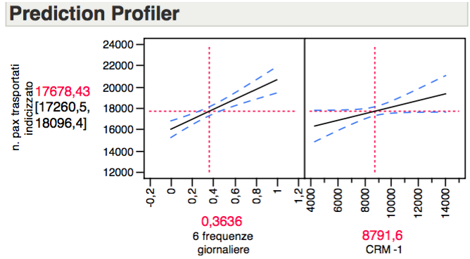
CONCLUSIONS:
The regression analysis conducted with the Backward Method, defines the daily frequencies and the Customer Relation Manager (CRM-1) significant variables in terms of explained variance in order to predict the number of passengers transported on the route from A to B.
More specifically, keeping constant the number of frequencies, an investment in CRM of 1000 € produces in the month after an increase of about 311 passengers on a monthly basis. Conversely keeping constant the investment in CRM, the increase of a rotation, which is equivalent to two frequencies, produces an increase of about 4,633 passengers on a monthly basis.
The equation can be considered fairly realistic both with respect to the variables compared and to the weights assigned to them.
Here, finally, the graph shows the inclination of the two variables and their correlation with the dependent variable.
Sempre saputo che Intrieri è un titolare di cattedra di ingegneria gestionale di compagnia aerea…
veramente un elaborato eccellente.
Non credo che esistano in circolazione simili prototipi.
Complimenti
Finalmente in Italia qualcosa di nuovo da studiare. OK
Grazie mille Giuseppe.